The significant expansion of crowdsourcing applications in the last decade, along with the vast availability of mobile phones and similar personal sensory devices, has inevitably generated a considerable amount of location data. The ability to transform locations into business value has triggered the interest of our data-driven economy in spatial data analysis. Geodata science has tapped its way into the emerging field of data-related solutions, expanding the reasoning behind such solutions to an additional dimension — a spatial dimension.
But, does location data simply add space to the existing challenges, or is it actually doing much more? Should space be observed as a single dimension, or is it much more complex, and how?
These, and similar, intriguing questions are buzzing around the global data community, making known problems unknown again, and making known solutions obsolete. To tackle the challenge and try to find the answers to some of these questions, our research team has taken a common trajectory data mining problem, and followed the steps, from data cleaning, over trajectory discovery to routing.
The results of this research, together with the conclusions, knowledge gained and obstacles encountered, are the main discussion topics of this article.
Problem set
A spatial trajectory is a sequence of chronologically ordered geographical coordinates generated by a moving object. A moving object could be any object that changes its location over time and is equipped with a tracking device: people, vehicles, vessels, animals, even natural phenomena, such as hurricanes, tracked via satellite/aerial imagery. Generating such a dataset is the easy part. If the question were, “What can be done with it?“, the answer would be very broad, and it would generally depend on the specific usage requirements and the domain of one’s interest. However, if the question were, “How to deal with it?“, the discussion could steer towards the common trajectory mining challenges.
The focus of this research is on How, rather than What, and the effort made is concentrated on recognizing and solving specific challenges using a real dataset of geo locations gathered from taxi vehicles and buses in Aracaju, Brazil.
Dig into the dataset
Similar to any other data science project, spatial data science projects start with dataset exploration. What is contained in the dataset, how is data structured or unstructured, what are potential anomalies and how they need to be transformed in order to result in business value, are important questions that have to be addressed early on. So let’s look at our dataset.
The dataset contains geo locations of buses and taxi vehicles gathered via the Android app, and comes organized in two data tables: one holds a list of trajectories with additional features such as speed, distance, rating, car or bus indicators, while the other one contains timestamped geo locations for each trajectory. The raw dataset contains 163 taxi and bus trajectories and a total of 18 107 locations. The table below gives a statistical view of these trajectories.

Overview of trajectories by type in terms of total number, average number of locations and average distance traveled
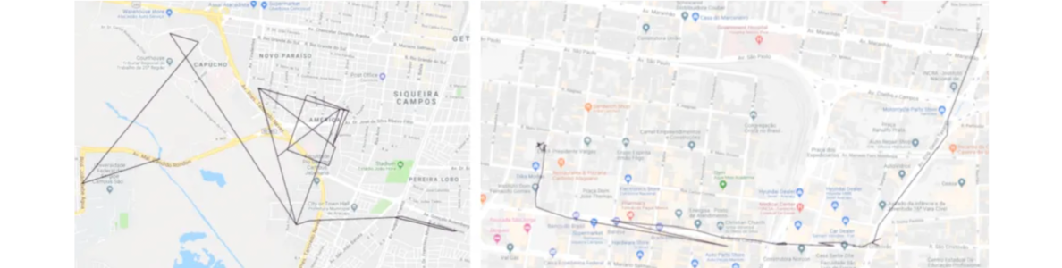
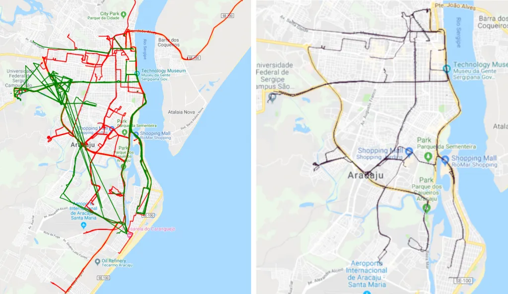
It is noticeable that the dataset is well balanced in terms of the number of examples per trajectory type (taxi or bus), while taxi trajectories dominate in terms of the average number of locations, and average distance traveled. The figure below shows the distribution of these trajectories on a map of Aracaju.
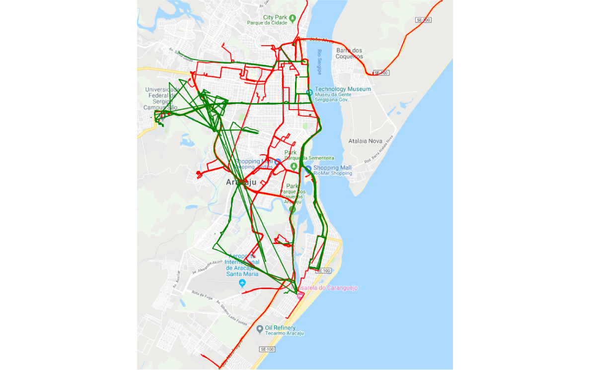
Distribution of taxi (red) and bus (green) trajectories on a map of Aracaju
The green lines represent buses, while the red ones show taxi vehicles. As expected, the taxi trajectories cover a wider area than the buses, which are usually limited to specific roads through the city. The visual exploration of a spatial dataset is the number one tool that should be used throughout the entire process as it could reveal the specificities in data behavior and point to either potential data problems or important features.
Data cleaning
Not a single data science project can be done without extensive dataset preprocessing. Real data is noisy, error-prone, incomplete and holds a certain amount of uncertainty. Moreover, it also comes in structures which are not fitted to specific business needs.
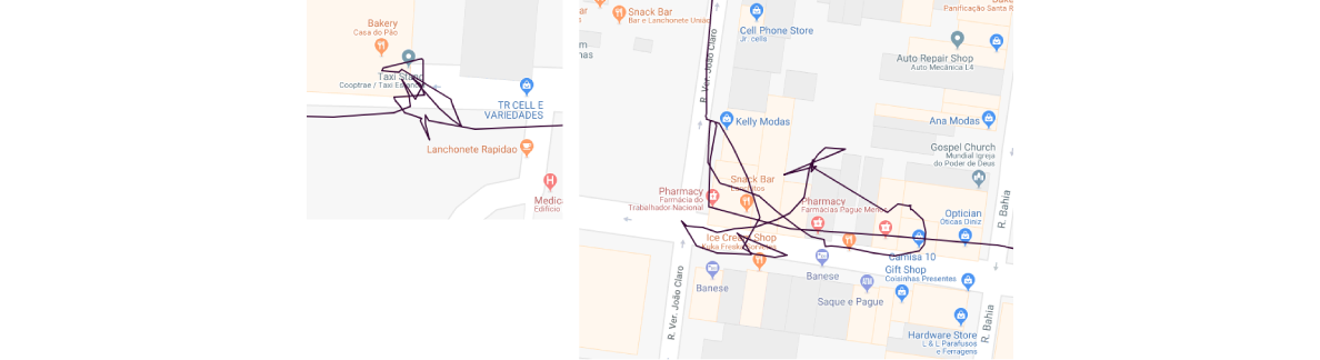
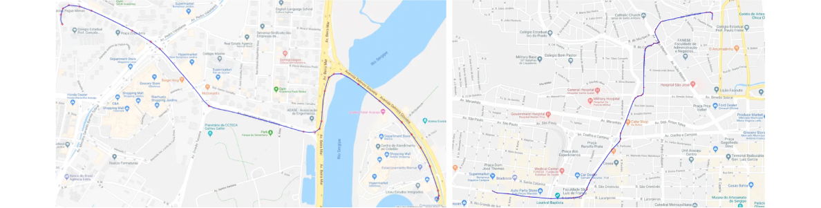
Looking at our dataset, and keeping in mind the final goal that needs to be achieved, it is noticeable that there are anomalous trajectories that do not carry useful information for road discovery. The examples can be seen in the following pictures.
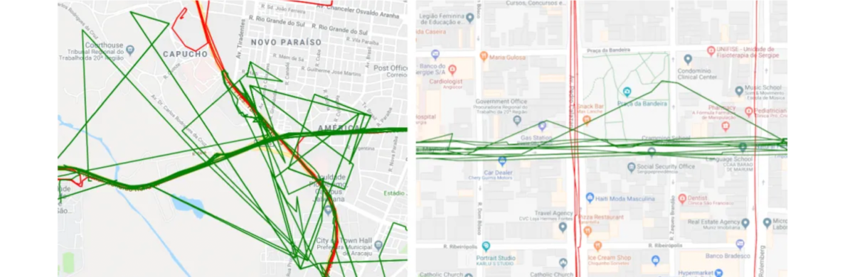
Examples of anomalous trajectories
The picture on the left gives an example of an anomaly that needs to be completely removed from the dataset. Such examples are a result of tracker inaccuracies over longer time periods and other known or unknown factors. As depicted, certain parts of the trajectory cross residential areas, which do not match real roads, and if kept for further processing they can only introduce a larger margin of error to the final solution.
The picture on the right demonstrates anomalies that could be corrected. These are also caused by tracker inaccuracies but are localized to a single point or a few close points in a trajectory. If successfully repaired, such trajectories could further be used in road discovery and later routing.
Various techniques can be applied to anomaly discovery and correction. Some propose map matching prior to any further processing, meaning that the trajectories are first being matched to a real road network and then processed further. This could be a good approach as it would enable easier recognition of road segments and potential anomalies; however, when dealing with large datasets, it could be time-consuming and probably inefficient. Other approaches are either based on using Kalman or semantic filtering.
The combination of semantic and Kalman filtering gave the best results for our dataset. The heuristic for detecting anomalies was considered to be focused either on distance or speed. For every two consecutive points in a trajectory, the distance between the points and the average speed were calculated. The goal was to identify larger scale anomalies, so, the threshold for distance was set to 300 meters and for speed to 120 km/h.
Once again, better results, in terms of the number of true anomalies detected, were achieved when considering only distance. A trajectory was completely discarded from the dataset if there was any segment with the distance larger than the threshold. The following are some of the discarded anomalous trajectories.
Examples of discarded anomalous trajectories
Although, the first thought would be to discard the entire trajectory, splitting it into a number of sub-trajectories based on the detected anomalies should definitely be considered. This could help preserve parts of the trajectory which are valid and useful for further road discovery. For the purpose of this experiment, the decision was made to simply discard them entirely.
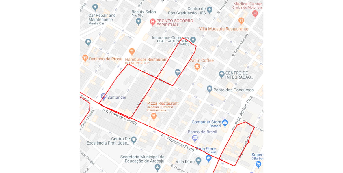
The next step was to detect complex trajectories, which are those that contain cycles. The approach undertaken here was to try to correct such trajectories by simply removing cycles without breaking their continuity. Those that could not be repaired were completely discarded. While this step helped detect and remove/repair anomalies that were not detected with previous semantic-based filtering, it also resulted in losing some of the valid trajectories. The lost ones were those going through city blocks and making valid cycles. A bit of a trade-off was made here because more was gained than lost with this approach, and the decision was reached that for the purpose of experimenting this step could be kept. However, when it comes to applying this approach to a real project, this step would either had to be revised or moved to a later phase where it could be applied to known segments, rather than the entire trajectory. Here are some of the examples of the detected and the removed complexities:
Examples of removed complex trajectories
And here is an example of the lost valid trajectories.
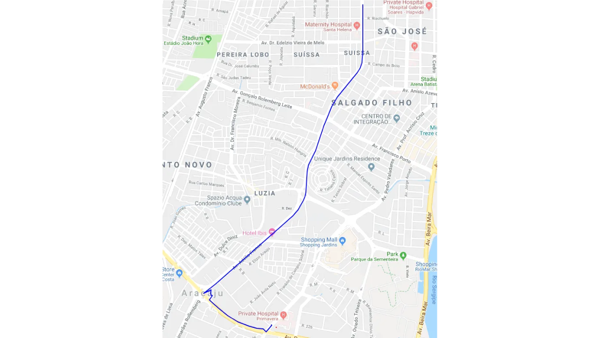
The last cleaning step was the smoothing of our trajectories by applying the Kalman smoothing algorithm. This approach helped detect and smooth out the localized peaks in trajectories, as depicted in the following images.
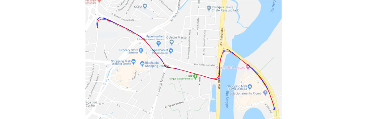

Application of Kalman smoothing algorithm. Blue lines represent original trajectory, while red ones represent smoothed result
The blue lines in the images represent the original trajectory, while red ones are the resulting trajectories after applying the Kalman smoothing algorithm.
After applying all of the data cleaning techniques described above, the dataset was reduced from 163 to 69 trajectories. More than 50% of the original trajectories were erroneous and discarded! Surprising? Not much actually. For anyone involved in data science, this number is not at all unexpected, but it does emphasize the importance of data preprocessing. Imagine the error that would have occurred if these anomalous trajectories were actually used.
Trajectory data mining
Trajectory data mining is not an unknown problem, but it is an issue that does not lose its popularity. This is probably because there is still no final solution for this problem set, and its popularity implies that a lot of different approaches have been tried and proposed. Segment clusterization is one of them and the one used in this research. It is convenient as it enables observing a set of trajectories as a set of their segments, without having to know anything regarding the architecture of the underlying road network (e.g., turns, stop points, intersections, etc.)
The general idea behind the segment clusterization is to divide each trajectory into representative segments and then identify those that are close enough to be merged together. Sounds easy, but what does it actually mean implementation-wise?
Trajectory segmentation
Trajectory segmentation is the problem of trajectory simplification. The main task here is to identify representative segments of a trajectory without corrupting its geometry. There are many reasons for this, among which the most important ones are reducing the computational complexity and getting more insights by focusing on the sub-problems (segments). Many techniques are available for trajectory segmentation, including those using time intervals, the ones focused on shape and the semantic-based techniques. For the purposes of road discovery, it is very important not to corrupt the shape of the trajectories. Therefore, the choice was set on the Douglas-Peucker algorithm as one of the shape-based segmentation algorithms. Trajectories must not be oversimplified so as not to change the shape significantly. Consequently, the parameters were set in a way to maximally preserve the original shape. The following are the examples of the results after applying this algorithm.
Examples of identifying representative segments after applying Trajectory Segmentation algorithm
The blue line on both images represents the original trajectory, while the red dots show the partition points identified by the algorithm. Each trajectory is broken down into segments, and only these segments are being considered in further processing. Out of 69 trajectories, a total of 1740 segments are identified.
Segment clusterization
Segment clusterization is another known problem, approached many times in many different ways. The idea is to find similar trajectory segments and group them together. But how can a similarity measure between segments be defined? Relying solely on the distance is very untrustworthy, as segments carry additional information which needs to be considered, such as direction. A good approach was proposed by the TRACLUS algorithm that redefines distance between two trajectory segments and proposes a density-based clustering approach for grouping similar segments.
The distance-based similarity between two segments is calculated against three different aspects: perpendicular, parallel and angular distance, as shown in the image below.

Components for calculating distance between to line segments
The first step is to determine the projection points by projecting the shorter segment onto the longer one. In the picture above, these points are denoted as Ps and Pe and are a result of projecting the start and the end point of the segment Lj onto the segment Li. The perpendicular distance is then calculated based on the perpendicular distances between the original and projected points of the segment Lj. The parallel distance is the measure of the overlapping extent of the two segments, while the angular distance is the one taking care of the direction between them. The combination of these three distances defines the similarity between the observed segments.
The proposed clusterization algorithm is density-based, which means it detects close segments using the described distance function and identifies dense areas which can be declared a cluster. It is based on the DBSCAN algorithm and parameterized with the size of the neighborhood of the potential cluster center, minimal number of segments in the neighborhood needed to declare a set of segments as a cluster, and an angle between segments. The angle is crucial as this is the parameter that separates the segments close to each other but heading towards opposite directions, or the segments changing directions in an intersection. This approach also detects the outliers, the segments which are too far from the cluster that could not be assigned to any cluster and represent anomalies that could not be detected during the data cleaning phase.
For our dataset, the total number of detected clusters was 567. The following images represent the results before and after the cleaning and clustering on one part of the road map.

The example of applying segment clusterization algorithm on a part of the road map. The image on the left shows the original trajectories before data cleaning and clusterization. The image on the right represents the final results on the same part of the map.
The image on the left is the original dataset before applying cleaning and clustering algorithms, while the image on the right is the result of the same map area after the described algorithms were applied. As can be noticed, the presented approach did manage to define a single line for each direction on the roadmap, solely based on the GPS locations collected from buses and taxi vehicles. As a direct consequence of the cleaning phase, some of the roads were lost. This is something that can be corrected by changing the cleaning approach in the ways discussed in the previous sections, or by applying the new ones. This really does depend on the specific outcome which needs to be achieved. The following images demonstrate our starting (image on the left) and ending point (image on the right).
Graph modelling and routing
Having generated a clustered model out of the representative trajectory segments, we can see the results of all the hard work, and have the actual business needs demonstrated.
To provide a routing solution, some kind of routing model needs to be implemented. Graphs belong to such models as they can precisely simulate the behavior and the connectivity of a road network. Clustered segments were used to construct a graph so that each segment became an edge of the graph that connects nodes made from the end points of the segment. This is a directed graph, which means it distinguishes A to B and B to A paths. For routing, any known graph-based path-finding algorithm can be used. The testing, for our example, was made using the A-star algorithm with the simple distance used for heuristics. Here is a result of one particular routing request.
An example of finding a route between two points in a generated graph
What was gained?
So, how is this different than a traditional routing solution based on a known road network and graph algorithms? As mentioned at the beginning of this article, geo data science sheds new light on familiar challenges, exposing them to new insights. In this particular case, the routing model is built using the historical data: geo locations and trajectories made by vehicles actually driving the roads. By including space, another feature was inevitably included, and that is the driving experience.
The road network generated from this dataset is experience-based, and it reflects the roads chosen by the drivers who drive there daily. This would resemble having a local sitting next to you while you are driving through an unknown city and giving you tips and tricks on how to best arrive at the desired destination. Instead of finding the shortest or fastest route, your navigation system would enable you to have the optimal route in terms of driving experience.
Spatial data can reshape the way we are looking at common problems. Combined with data science, adding Where to When and How can become a powerful tool for reinventing the way we understand data diversity. Trajectory data mining is the perfect example, and its popularity emerges exactly from the diversity of the underlying problems it could be applied to.
Experience-based routing, maritime routing, route recommendation, or combination with other semantic data sources for behavior pattern discovery, such as detecting events of interest, are just some of the examples whose application mostly depends on the specific business use cases. However, once the methodology for mining trajectories from a cloud of locations is conquered, the application possibilities are practically endless.